Chapter 4: Architecture Design
Typical system topology, device interconnection, communication architecture, and power design for environmental noise monitoring networks
A well-designed system architecture is the foundation of a reliable, scalable, and maintainable environmental noise monitoring network. Architecture design encompasses the physical topology of monitoring stations, the communication pathways between field devices and the management platform, the power supply strategy, and the data flow from raw acoustic measurements through processing, storage, and reporting. This chapter presents the canonical three-tier architecture used in professional ENMS deployments, illustrates a typical device wiring configuration, and provides guidance on selecting the appropriate architecture variant for different project scales and regulatory requirements.
4.1 Three-Tier System Architecture
Professional environmental noise monitoring systems are organized into three functional tiers: the Field Layer containing measurement hardware, the optional Edge Layer providing local aggregation and pre-processing, and the Platform Layer hosting the cloud-based data management and reporting infrastructure. This layered approach separates concerns, enables independent scaling of each tier, and provides resilience through local buffering when connectivity to the platform is temporarily unavailable.
1Field Layer
Monitoring stations with Class 1/2 instruments, microphones, DSP units, power systems, and cellular/fiber uplinks. Each station operates autonomously with local data buffering.
2Edge Layer (Optional)
Local gateway devices aggregating data from multiple nearby stations, performing pre-processing, protocol translation, and providing a local network access point for maintenance.
3Platform Layer
Cloud-hosted management platform providing data ingestion, QA/QC processing, time-series storage, alerting, GIS visualization, regulatory reporting, and API integration.
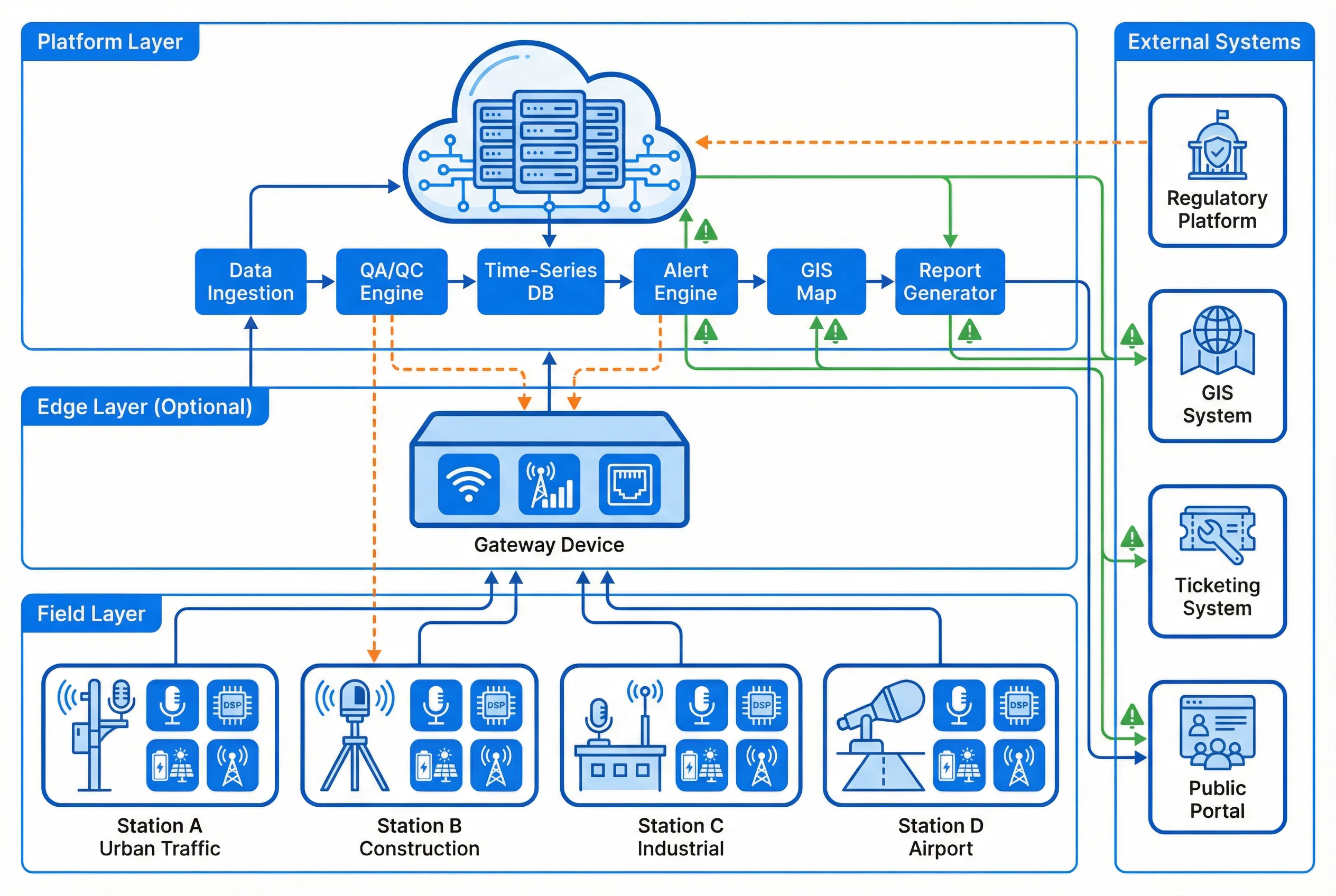
Figure 4.1: Typical three-tier ENMS topology showing Field Layer stations, optional Edge Layer gateway, Platform Layer components, and external system integrations
The topology diagram illustrates four representative field stations (urban traffic, construction, industrial, and airport) communicating via cellular or fiber connections to the platform layer. The platform layer processes incoming data through a sequential pipeline: Data Ingestion validates packet integrity and timestamps; the QA/QC Engine applies meteorological flags, calibration corrections, and outlier detection; the Time-Series Database stores validated measurements; the Alert Engine evaluates threshold conditions and dispatches notifications; the GIS Map provides spatial visualization; and the Report Generator produces regulatory submissions. External system integrations include the regulatory authority platform, GIS systems, ticketing/complaint management systems, and public information portals.
4.2 Communication Architecture
Communication design must balance reliability, latency, bandwidth, cost, and security requirements. The table below summarizes the primary communication technologies used in ENMS deployments and their appropriate application contexts.
| Technology | Bandwidth | Latency | Coverage | Cost | Best For |
|---|---|---|---|---|---|
| 4G LTE | 10–100 Mbps | 20–50 ms | Urban/suburban | Medium | Urban traffic, construction, entertainment |
| 5G NR | 100 Mbps–1 Gbps | 1–10 ms | Dense urban | High | High-density networks, real-time audio |
| Fiber Ethernet | 100 Mbps–10 Gbps | <1 ms | Fixed locations | High install | Airport, industrial, permanent fixed stations |
| WiFi 802.11 | 54–600 Mbps | 5–20 ms | Short range ≤100 m | Low | Campus, school, hospital, temporary |
| Satellite (LEO) | 10–200 Mbps | 20–100 ms | Global | High | Remote, nature reserve, off-grid |
| LoRaWAN | 0.3–50 kbps | 1–5 s | Urban 2–5 km | Very low | Low-data IoT sensors, battery-powered nodes |
| NB-IoT | 20–250 kbps | 1–10 s | Wide area | Low | Low-power, low-data remote sensors |
Dual-Path Redundancy: For enforcement-grade and regulatory-reporting stations, always configure a primary and backup communication path. A typical configuration uses fiber as primary with 4G LTE as backup, or dual-SIM cellular with automatic failover. The station must buffer data locally during connectivity loss and upload the backlog upon reconnection, with gap-free data continuity verified by sequence numbers or timestamps.
4.3 Station Wiring and Device Interconnection
The device wiring diagram defines the physical connections between all hardware components within a monitoring station enclosure. Correct wiring is critical for measurement accuracy, electromagnetic compatibility, and long-term reliability. The diagram below shows the complete wiring configuration for a standard solar-powered cellular station, including all input and output interfaces of the noise monitor controller.
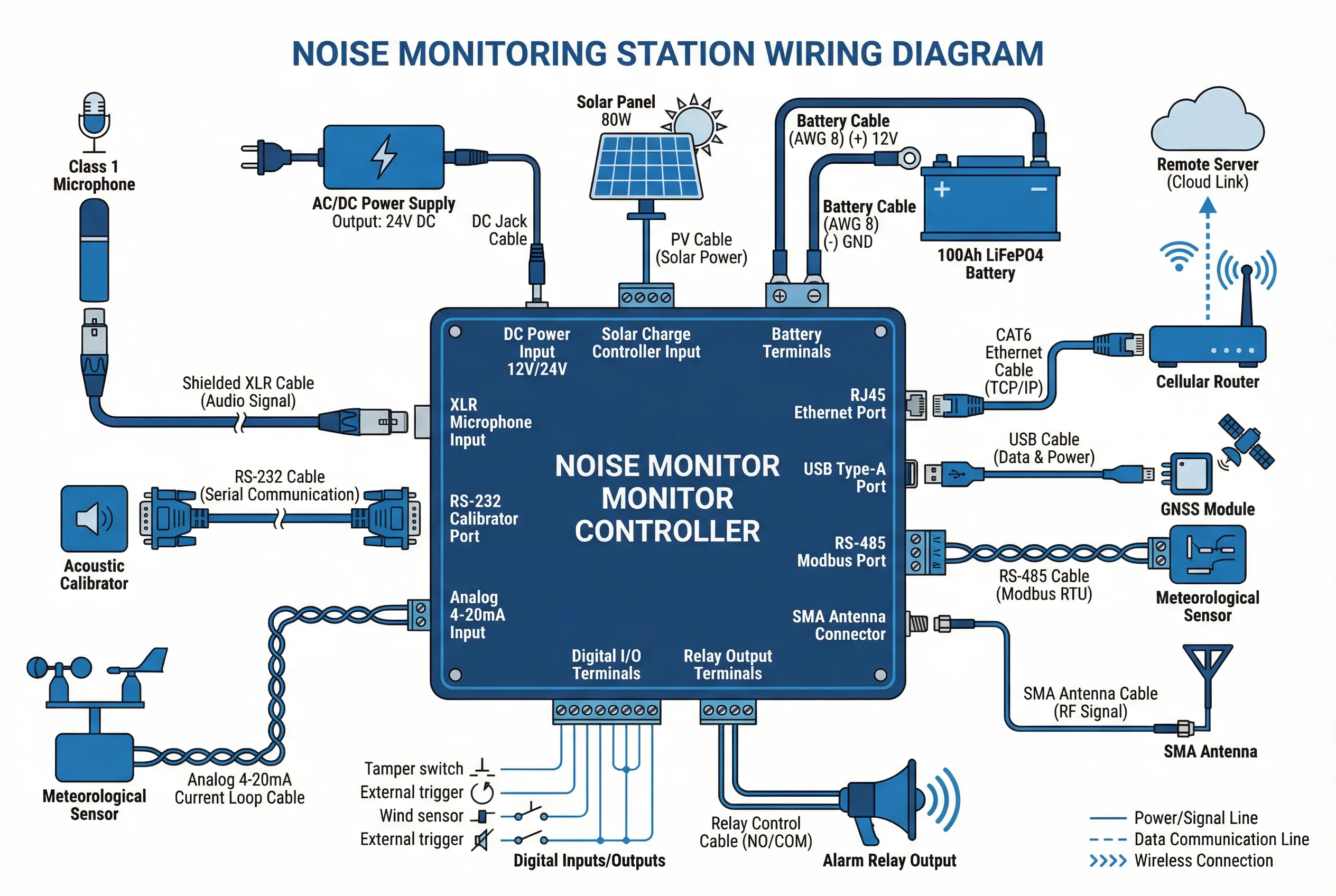
Figure 4.2: Complete device wiring diagram for a solar-powered cellular noise monitoring station, showing all input/output connections, cable types, and protocols
The wiring diagram highlights several critical design principles. The microphone connects via a shielded XLR cable to minimize electromagnetic interference pickup along the cable run from the outdoor microphone to the indoor controller. The RS-485 Modbus bus connects meteorological sensors using twisted-pair shielded cable with proper termination resistors at both ends. Power wiring uses appropriately sized conductors (AWG 8 for battery cables) to minimize voltage drop and heat generation. All cable entries into the enclosure use IP-rated glands to maintain the weatherproof rating. Relay outputs for alarm signaling use normally-open (NO) contacts to fail-safe in the de-energized state.
| Interface | Protocol | Cable Type | Max Length | Notes |
|---|---|---|---|---|
| Microphone Input | Analog XLR balanced | Shielded 2-core + screen | 50 m | Low-impedance, phantom power optional |
| Calibrator Port | RS-232 serial | Shielded multi-core | 15 m | Used for auto-calibration sequences |
| Met Sensor Bus | RS-485 Modbus RTU | Shielded twisted pair | 1200 m | 120Ω termination at each end |
| Analog Input | 4–20 mA current loop | Shielded 2-core | 300 m | For legacy sensor integration |
| Network Uplink | Ethernet TCP/IP | CAT6 FTP | 100 m | To cellular router or fiber media converter |
| GNSS Module | USB / UART | USB cable or coax | 5 m USB / 30 m coax | Active antenna requires coax feed |
| Solar Input | DC PV cable | 6 mm² PV cable | 10 m | UV-resistant, rated for outdoor use |
| Battery | DC power | AWG 8 / 6 mm² | 2 m | Fused at battery terminal |
| Relay Output | Dry contact NO/NC | 2-core signal cable | 100 m | Max 250V AC / 5A switching |
4.4 Power Architecture Design
Power architecture is a critical design dimension that directly affects system availability, maintenance burden, and total cost of ownership. The appropriate power strategy depends on grid availability, solar irradiance at the deployment location, required autonomy during cloudy periods, and the power consumption profile of the installed equipment.
| Power Configuration | Components | Typical Autonomy | Best Application | Relative Cost |
|---|---|---|---|---|
| Grid AC only | AC/DC PSU + UPS battery | 4–8 h (UPS) | Urban fixed stations with reliable grid | Low |
| Solar + Battery | Solar panel + MPPT + LiFePO4 | 3–7 days | Remote, construction, temporary | Medium |
| Grid + Solar backup | Grid primary + solar + battery | Indefinite (grid) + 3 days | Critical enforcement stations | Medium-High |
| Solar + Wind + Battery | Solar + wind turbine + large battery | 7–14 days | Remote, high-latitude, nature reserve | High |
| PoE (Power over Ethernet) | PoE switch + CAT6 cable | Depends on switch UPS | Campus, school, short cable runs | Low |
For solar-powered deployments, the battery capacity must be sized to provide the required autonomy during the worst-case consecutive cloudy days at the deployment latitude. A standard sizing methodology uses the formula: Battery Capacity (Ah) = (Daily Load (Wh) × Autonomy Days) / (System Voltage × DoD × Battery Efficiency). For a typical station consuming 15 W continuously (360 Wh/day) requiring 5 days autonomy at 12V with 80% DoD and 95% efficiency, the required capacity is approximately 200 Ah. LiFePO4 chemistry is strongly preferred over lead-acid for its superior cycle life (2000+ cycles vs. 300–500), wider operating temperature range, and stable discharge voltage.
4.5 Data Flow and Processing Architecture
The data processing pipeline within the platform layer transforms raw acoustic measurements into validated, actionable environmental noise data. Each stage of the pipeline applies specific processing logic that must be understood and configured correctly during system design.
| Pipeline Stage | Input | Processing | Output | Key Parameters |
|---|---|---|---|---|
| Data Ingestion | Raw packets from stations | Packet validation, deduplication, timestamp normalization | Validated time-stamped records | Sequence number check, CRC validation |
| QA/QC Engine | Validated records | Met flags, calibration correction, range check, outlier detection | Flagged and corrected data | Wind speed threshold, calibration drift limit |
| Aggregation | 1-second or 1-minute data | LAeq calculation, percentile statistics, spectral averaging | Hourly, daily, period statistics | Averaging period, weighting network |
| Alert Engine | Aggregated statistics | Threshold comparison, exceedance counting, notification dispatch | Alerts, SMS, email, API webhook | Threshold levels, alert delay, escalation rules |
| Time-Series DB | All processed data | Indexed storage, compression, retention policy enforcement | Queryable historical archive | Retention period, compression ratio |
| Report Generator | Historical data queries | Statistical computation, chart generation, regulatory format export | PDF/CSV/XML reports | Report template, regulatory standard, time period |